In computer science, the maximum subarray problem is the task of finding the contiguous subarray within a one-dimensional array of numbers which has the largest sum.

Chapter 4 of the CLRS text uses the maximum subarray problem as an example of an algorithm that can be solved using the divide and conquer paradigm. It turns the maximum subarray problem into a recurrence almost identical to that of merge sort being of $O(n\log(n))$ time complexity.

In this post, I’m going to talk briefly about two $O(n)$ dynamic programming solutions and some of the intuition behind them. I’ll then touch on some of the performance tests I ran between three solutions:

• Naive $O(n^2)$ time complexity
• Divide and conquer $O(n\log(n))$ time complexity
• Dynamic programming $O(n)$ time complexity

Dynamic Programming

As per the norm with just about any dynamic programming problem, we want to maintain some structure of optimized subproblem answers to help us solve larger problem instances. First, we need to define the state of the subproblem. Then we need to forge a relationship between the original problem and the subproblem so we can see how we’ll extend the answers in our dp structure. Eventually, we want to return the sum of the maximum subarray within $A[0 \ldots n]$.

Common DP Patterns

A natural approach is to frame the subproblem as a straight recursive definition. This means we want to figure out if we can relate the sum of the maximum subarray within $A[0 \ldots i]$ to the sum of the maximum subarray within $A[0 \ldots i-1]$. Our dp array would contain sums of maximum subarrays within $A[0 \ldots k] \forall \; k \in \{ 0 \ldots n-1 \}$. The array would then be some non-decreasing series with the answer to our original problem sitting at the end. This sort of tabulation is a fairly common dp pattern. Unfortunately, we can quickly show that our idea of a subproblem doesn’t easily relate to instances of a larger size. For example, if $A[0 \ldots i-1]$ was the following array:

with our current model our dp array would look like:

It is true that the sum of the maximum subarray within $A[0 \ldots i-1] = 300$, no matter how many values negating this sum come after the end of the actual maximum subarray $[100, 200]$, which lies somewhere inside $A[0 \ldots i-1]$. Consequently, we cannot easily extend our subproblem’s answer to a larger instance. This is because we don’t know how many detrimental numbers we may be forced to accept in order to bridge the gap between the end of the true maximum subarray, and some newly introduced number $A[i]$. Put differently, there’s no guarantee that the last number of the subproblem is contained in its maximum subarray.

In order to see how a previous subproblem can be extended, we need to know how the last element is going to affect the element we’re introducing. We need to know the sum of the maximum subarray ending with element $A[i-1]$. Then we can introduce $A[i]$ and decide whether it is beneficial to tack on $A[i]$ to the subproblem, or if we’d be better off counting $A[i]$ separate (if previous subproblem sum is negative). This relation between subproblems and larger instances becomes more clear and our dp array will be used to store the sum of the maximum subarray ending with element $k \; \forall \; k \in \{ 0 \ldots n-1 \}$. The dp array for the above example would look like this:

Then when we introduce $A[i]$, we know we don’t want to add it to the maximum sum of the subarray ending in $A[i-1]$ because we’d already be starting the sum at $-500$. We’ll only want to add $A[i]$ to the previous maximum sum if that sum is positive. Our dp array will then consist of peaks and valleys where the answer to our original problem is the largest of these peaks. We can maintain a variable whose value only gets updated when we see a new maximum value in the dp array, so we can return it right when we get to the end. This is another common dp pattern differing slightly from keeping a non-decreasing array of subproblem values.

$\Theta(1)$ space complexity optimization

We can further optimize the solution for $O(1)$ space complexity by realizing that to solve the problem for $A[0 \ldots i],$ we only need the value of the last subproblem and no data prior to it. The other tabulated subproblem answers are useless after they’ve been used once. This should tell us we can replace the array of subproblems with two variables maxSum and currentSum. currentSum acts as the ever-changing $dp[i-1]$, keeping track of the current maximum subarray ending in $i-1$. Every iteration we then update currentSum when we evaluate $A[i]$. We then update maxSum to be the larger of the two variables. Once we have the maximum value saved, we then send currentSum back to the trenches. By the end of the array, the currentSum could very well be the smallest it’s ever been, but as long as maxSum has captured the value of currentSum at its highest value that’s all we need to return. The C++ code for this problem is as follows:

/**
 * This algorithm embodies
 * the technique of keeping track
 * of the maxSubarray we have come
 * accross thus far. This gives us a
 * one-pass O(n) solution
 */
tuple<int, int, int> maximumSubarrayLinear(vector<int> &nums) {
  if (!nums.size()) return make_tuple(0, 0, 0);
  int startIndex, endIndex, currentStartIndex, currentEndIndex;
  int maxSum = INT_MIN, currentSum = 0;

  for (int i = 0; i < nums.size(); ++i) {
    if (nums[i] > currentSum + nums[i]) { // if (currentSum < 0) ex: [-200, 5] sum of maxSubarray = 5, not -195
      // Start the 'current' subarray at a new index
      currentStartIndex = i;
      currentSum = nums[i];
    } else {
      // Update new 'current' subarray ending index
      currentEndIndex = i;
      currentSum = currentSum + nums[i];
    }

    if (currentSum > maxSum) {
      startIndex = currentStartIndex;
      endIndex = currentEndIndex;
      maxSum = currentSum;
    }
  }

  return make_tuple(startIndex, endIndex, maxSum);
}

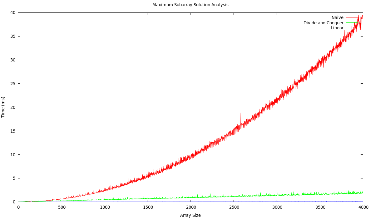
Quick performance study

A quick performance study of three solutions for this problem yields the expected results, given the time complexity for each solution. The vector each solution worked on contained random values ranging from $0-20,000$ with a $33$% chance the value was negative. The maximum size of the vector was $4,000$ elements. I originally did a max of $10,000$ elements, however, the naive $O(n^2)$ solution smashed the other solutions to the bottom of the graph due to its inefficiency. So I lightened it up a bit.